what kind of information is indicated by the graph of the acceleration due to gravity
The following is suggested as a possible beginning example, for students, of numerical integration.
The phenomenon of a falling ball, accelerating at close to ten grand s-2 , can speedily be given a graphical solution. Knowing that the altitude fallen is given by south = ½a t 2 likewise makes information technology possible to bank check the graphical technique.
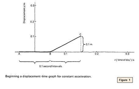
Suppose the ball starts at remainder, at time t = 0. Over a short time, say 0.1 second, around t = 0 the velocity is pretty well naught, the altitude travelled is besides nearly zero, and the first chip of the graph must be flat, similar the segment AB in the figure above.
But in the following interval of some other 0.1 second, around the 'time-of-mean solar day' t = 0.one 2nd the average velocity will equal that at that time. If the acceleration is 10 metres per 2d each second, the velocity is 1.0 metre per 2nd. So the adjacent segment of the graph, BC, in the same figure, rises or slopes up at one.0 metre per second, ascension in all 0.1 metre in an interval of 0.one second.
The next 0.1 2nd interval centres effectually the time 0.2 second from the showtime, when the velocity will be averaging 10 10 0.2 = ii metres per second. So the next section of the graph slopes up twice as steeply, rising 0.2 metre over 0.1 s econd. And so information technology goes on. The rule is easy: around each time t describe a section of line for velocity x t which must rise an extra distance (0.one) 10 t metre.
Annotation that for successive equal fourth dimension intervals Δt, the velocity rises past the same amount each time. The acceleration is constant.
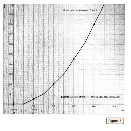
Such a graph is shown in a higher place (figure 2). The circles marker points calculated from south = ½a t 2 , for comparison. It predicts, for case, that a heavy brawl volition fall ane metre in 0.45 2nd. This could be tested using a scaler to time the fall, if your course feels the need. Or a ball could simply be dropped, and the class be asked to judge the time. The equation s = ½a t 2} and the kinked bend
are both solutions
of the equation:
dispatch = 10 chiliad south-two or, better, of = a where a = 10 one thousand s-two .
The graph is an QuoteThis{guess solution: it is near to the exact solution, and although where it is incorrect it always makes the distance come up out a little too small, the graph does not drift off grade (that is, the errors do not accumulate). The smaller the interval Δt, the ameliorate the approximation. When solving existent problems in this style, engineers and physicists devote much attention to choosing Δt small enough to be just sufficiently accurate, but not so small-scale as to make the chore unnecessarily slow. Students are probable to have more than conviction in the idea if the problem of 'sufficiently good' approximations is taken seriously.
(Tin can whatsoever standard school-level apparatus, in fact, detect an error of the size there appears to be between the graph and results found from s = ½a t 2 ?)
How constant acceleration is represented in drawing the graph
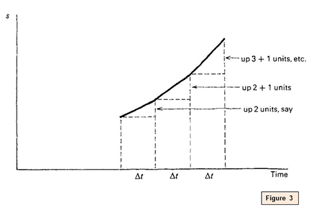
See figure three above. In cartoon the graph, each new section was drawn at a steeper slope; that is, a larger velocity. Because the acceleration was constant, the slope increased by equal amounts in each stride.
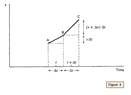
See figure 4. At each moment the average velocity virtually that moment was worked out, using a = x m s-ii . A line like AB in the above figure at the correct slope was put in, going an extra distance vΔt. At the side by side moment, v was larger, say v + Δfive, where v is the actress velocity gained in an interval Δt. A line such equally BC was drawn, at the new, larger slope, going a larger extra distance (v + Δv) Δt.
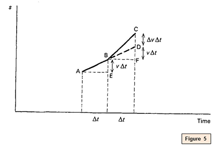
If, as in effigy 5, AB is run on at the same slope, to D, then DF = 5Δt is the extra distance that would have been covered if the velocity had non increased. The actress extra
bit CD = ΔvΔt is the 'actress actress distance' gone considering the velocity did increase, by Δfive.
So CD = Δ5Δt = a(Δt)(Δt) = a (Δt) 2
A dominion for drawing graphs of acceleration
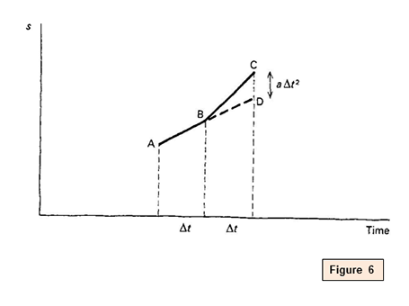
Looking at effigy 6, at that place is a uncomplicated dominion for drawing acceleration graphs. Take the graph AB as found at the last interval, and run on AB directly to D, as if there were no acceleration. Then add an extra extra distance
DC, where DC = a (Δt) 2. So BC is the side by side bit of graph. If the acceleration should vary, the actress extra distances
similar DC will vary; just piece of work them out from the basic recipe.
The rule with a Δ notation
For some students, the argument in terms of acceleration volition be more plenty. But others may like to see how the calculus notation is useful. Δ is used to hateful pocket-sized change in . . .
.
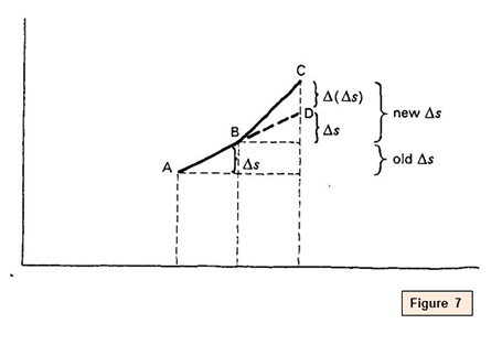
Over AB, in figure 7, the velocity v is the gradient of AB, that is Δs Δt . Then the velocity rises, and the acceleration is
Over the timeΔt, the distance s changes by more than it would take changed if at that place had been no dispatch, and Δs in the second interval is larger than Δsouth in the beginning by the 'extra actress distance' Δ(Δs). Farther, the dispatch is Δ(Δs) Δt two , equal to the charge per unit of change of velocity around B.
Then the rule remains the same: add on an 'extra extra distance' over and to a higher place that which would come from taking the graph straight on. The size of the 'extra actress distance' should be:
Δ(Δs) or Δ2 s = (acceleration)Δt 2.
Δsouth Δt approximates to the velocity v, or dsouthward dt .
Δ2 s Δt 2 approximates to the acceleration a, or d 2 southward d t 2 .
Source: https://spark.iop.org/collections/acceleration-due-gravity
0 Response to "what kind of information is indicated by the graph of the acceleration due to gravity"
Post a Comment